Hypothesis Testing in Practice: A Developer’s Guide

At 2 a.m., a checkout refactor reaches production. Grafana shows conversion moving upward, latency looks acceptable, and the team starts discussing rollout. Then someone asks the uncomfortable question: did the code improve checkout, or did the last hour just contain an unusually favorable slice of traffic?

That question is the practical heart of hypothesis testing. Engineers use it to separate a plausible signal from ordinary variation, but a test isn’t a machine that turns uncertainty into truth. It helps you make a better decision when paired with a clear metric, sound experimental design, effect-size analysis, and knowledge of how the system behaves under real traffic.

Why Hypothesis Testing Matters for Engineers

Dashboards are excellent at showing that something changed. They aren’t, by themselves, good at explaining whether the change came from your release, traffic composition, delayed events, or random fluctuation.

Suppose the checkout refactor appears faster and conversion rises. A hypothesis test gives the team a disciplined question to ask: if the refactor had made no real difference, how surprising would these observations be? That reframing replaces “the graph went up” with a decision rule the team can inspect and challenge.

Three decisions that need more than a dashboard

First, a feature can look faster while increasing payment errors. A latency panel may encourage a launch, while an error-rate guardrail argues against it. Testing the relevant outcomes together prevents the team from treating one attractive metric as the whole product experience.

Second, a release can look slower during an unusual traffic window. Rolling it back immediately might discard a sound change. Comparing the release with a defined baseline, while accounting for variation in the measurement, helps distinguish a transient observation from evidence of a regression.

Third, a postmortem may leave two fixes that are equally plausible. One engineer blames connection pooling, another suspects a serialization change. Rather than allowing seniority or intuition to settle the debate, the team can turn both explanations into measurable hypotheses and design a comparison.

Practical rule: A dashboard tells you what happened. A hypothesis test helps you decide whether the observed difference is compatible with the baseline you expected.

The value isn’t limited to formal research. It appears whenever an engineering team must choose whether to ship, roll back, investigate, or collect more evidence. A useful test makes the assumptions visible: what counts as a meaningful outcome, which observations belong in the comparison, and what evidence would change the decision.

That discipline also exposes weak questions. “Did the new checkout work better?” is too broad. “Did the new checkout change completion rate without worsening payment errors or latency?” gives the team outcomes it can measure and constraints it can defend.

The Core Statistical Concepts You Actually Need

Use one running example. Your team changes the checkout flow and wants to know whether the treatment changes checkout completion rate.

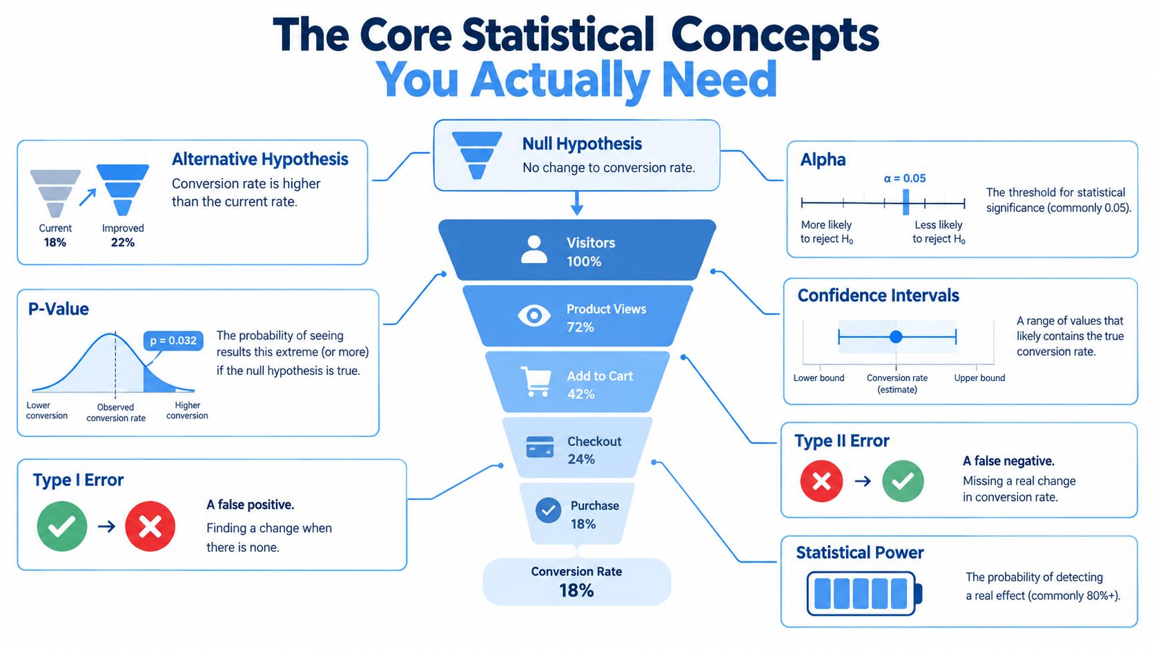
The null hypothesis is that there’s no change in checkout completion rate. The alternative hypothesis is that the treatment changes the rate in the direction your team cares about, such as an improvement. You should write these statements before looking at the result, because otherwise the result can reshape the question.

Set the decision language first

Choose a significance level, often called alpha, before collecting or inspecting the data. In this example, set alpha to 0.05. That threshold represents the false-positive tolerance built into the test, not the probability that your product idea is correct.

A p-value answers a narrow question: assuming the null hypothesis is true, how likely is it that you’d observe data this extreme or more extreme? A small p-value indicates that the data would be unusual under the no-change model. It doesn’t tell you the probability that the null is true, and it doesn’t measure business value.

The result should also include an effect estimate and a confidence interval. If the treatment appears to change completion rate, the interval describes a range of effect values compatible with the analysis and its assumptions. A narrow interval near zero tells a different product story from a wide interval that includes both a worthwhile improvement and a harmful regression.

Connect errors to engineering costs

A Type I error is a false positive. You conclude that the refactor changed checkout when the apparent difference came from noise, then ship a change that doesn’t deliver the expected benefit. A Type II error is a false negative. The refactor really helps, but the test fails to detect it, so the team keeps a less effective implementation.

Statistical power is the ability of a test to detect an effect of a specified size under a chosen design. Power depends on factors such as sample size, variability, and the effect you want to detect. A small dataset can make a useful change difficult to distinguish from noise, while a very large dataset can make a tiny effect look statistically persuasive.

The authoritative discussion of statistical significance and practical meaning makes the central caution clear: a small p-value doesn’t prove that an effect matters in practice, and a non-significant result doesn’t prove that no effect exists. Pair the test with confidence intervals, effect sizes, and a domain threshold that answers, “Would this change justify engineering and operational cost?”

Write the decision before running the test:

1. Outcome: checkout completion rate, plus latency and error guardrails.
2. Null: no change in completion rate.
3. Alternative: the treatment improves or worsens completion rate, depending on the directional question.
4. Threshold: alpha equals 0.05, alongside a practical effect threshold.
5. Action: ship, hold, roll back, or gather more evidence.

That structure keeps “not statistically significant” from becoming the misleading conclusion “the treatment has no effect.” It may mean the data are too noisy, the design has limited power, or the plausible effect range includes outcomes the business treats as equivalent.

Choosing the Right Test for Your Data

The test follows the shape of the data and the way observations were collected. Start with the outcome, identify whether observations are independent, then check whether the assumptions of the candidate method are credible.

Test	Data Shape	Typical Use Case
t-test	Continuous measurements, with assumptions about the mean and distribution	Comparing page render time between two independent variants
Chi-square test	Counts across categorical outcomes	Comparing checkout completions and non-completions between variants
Bootstrap	Resampled observations from an empirical dataset	Estimating uncertainty for skewed latency or an awkward statistic
Permutation test	Exchangeable observations under a null model	Comparing groups when distributional assumptions are uncertain

Match the method to the question

A t-test earns its place when the metric is continuous, such as render time, and the comparison concerns a difference in means. In Python, a basic independent comparison might look like:

scipy.stats.ttest_ind(control_latency, treatment_latency, equal_var=False)

The Welch form avoids assuming that both groups have the same variance. It still doesn’t solve dependence, repeated users, instrumentation bias, or a heavy-tailed metric by itself.

For checkout conversion, the raw data are categorical counts. A chi-square test can compare a table of treatment status against completion status:

scipy.stats.chi2_contingency([[completed_control, incomplete_control], [completed_treatment, incomplete_treatment]])

That result should sit beside the estimated difference in conversion and its interval. A test statistic without the size and direction of the effect is difficult to use in a product decision.

A bootstrap repeatedly resamples observed records to approximate the distribution of an estimator. It can be useful for a percentile, ratio, or skewed latency summary that doesn’t fit a convenient textbook formula:

numpy.percentile([np.mean(np.random.choice(latency, size=len(latency), replace=True)) for _ in range(B)], [2.5, 97.5])

The code is a sketch, not a complete analysis. You still need to choose a resampling unit, preserve user-level dependence, and define the statistic before running it.

A permutation test builds a null distribution by shuffling group labels when the exchangeability assumption is reasonable:

scipy.stats.permutation_test((control_latency, treatment_latency), statistic, permutation_type='independent')

Use a checklist before selecting anything:

• Counts: Start with a categorical method for conversion outcomes.
• Means: Consider a t-test when independent observations and its assumptions are defensible.
• Skewed distributions: Examine quantiles and consider bootstrap or a resistant comparison.
• Paired observations: Use a paired method, not an independent-group test.
• Repeated users or sessions: Model the dependence or aggregate at the appropriate unit.
• Unclear assumptions: Prefer an explicitly justified resampling approach over selecting a familiar test automatically.

A flexible test isn’t automatically a better test. The strongest choice is the one whose assumptions match how your application generated the data.

Running Hypothesis Tests in Software QA

QA can use hypothesis testing before a change reaches customers. Treat the regression baseline as the null state and the proposed fix as the alternative. For a checkout bug, the question might be whether the fix restores successful completion without introducing latency or error regressions.

Turn the test plan into a measurable contract

Start by identifying the input and output. If the fix changes whether users complete checkout, collect completion and non-completion counts. If it changes a request path, collect latency observations and error outcomes. The test should reflect the failure mode, not whichever metric is easiest to export.

QA Question	Hypothesis Form	Recommended Test	Required Inputs
Did the fix change completion behavior?	Null says outcome proportions match the baseline	Chi-square test	Completion counts by build
Did the refactor change request latency?	Null says latency means are equal	Welch t-test, or a resampling method if assumptions are weak	Independent latency observations
Did the same test cases improve?	Null says paired differences center on no change	Paired test or paired permutation test	Matched observations by case
Did failures cluster in a category?	Null says category and outcome are unrelated	Chi-square test	Category-by-result counts

Pre-register the thresholds and collection plan in the QA ticket before the run. Record which build is the baseline, which build is the candidate, how retries are handled, what constitutes a failed request, and which observation is the unit of analysis. This prevents a team from changing the rules after seeing an inconvenient result.

A deterministic test remains preferable when the system allows it. If the same input should always produce the same output, assert that directly. Statistical testing belongs where behavior includes timing, scheduling, concurrency, randomized recommendation, or other variation that a fixed assertion can’t represent.

Know where synthetic QA stops

A staging environment may have clean fixtures, different caches, different request mixes, and different downstream behavior from production. A refactor can pass deterministic tests and still fail when real sessions exercise an unanticipated sequence.

That gap doesn’t make statistical QA useless. It tells you what question the test answers. A staging comparison can establish that the candidate behaves as expected under the designed workload. It can’t automatically establish that the candidate will behave the same way under production traffic.

Capture the raw observations and test against a known baseline. If the result is inconclusive, don’t label the build safe or broken without qualification. Mark what remains uncertain, then use a more realistic workload, targeted instrumentation, or traffic replay to narrow the uncertainty before exposing users.

Designing A/B Experiments With Real Traffic

A recommendation team changes ranking logic to improve product discovery. The success metric is a downstream engagement event, while guardrails include response latency, error rate, and resource saturation. The team doesn’t begin by splitting every user. It first writes the hypothesis, identifies the randomization unit, estimates the required sample size, and states what result would justify rollout.

Randomization matters because the treatment and control groups need comparable opportunities to experience the change. Sample size estimation matters because the team needs enough information to distinguish a meaningful effect from ordinary variation. The decision rule should include both statistical evidence and practical thresholds, not just a pass or fail based on one p-value.

Rehearse the change before the experiment

Before real users see the candidate, the team can capture representative HTTP traffic and replay it against an isolated candidate service. GoReplay provides a record-and-replay mechanism for sending captured production HTTP requests into a testing environment, which lets engineers examine behavior using request patterns that synthetic fixtures may miss. The team can compare status codes, response payloads where appropriate, latency distributions, and error behavior while production continues serving users.

The sequence looks like this:

1. Capture: Record eligible requests while protecting sensitive data and defining which routes belong in the analysis.
2. Prepare: Route the replay to the candidate build and control timing, concurrency, and downstream dependencies.
3. Compare: Align candidate observations with the baseline and inspect errors, latency, and behavioral outputs.
4. Decide: Fix defects, adjust capacity, or proceed to a carefully controlled live experiment.

For implementation details, the GoReplay guide to replaying production traffic for realistic load testing is a useful reference. Teams exploring adjacent analytical careers may also find this overview of high-impact motorsport analytics roles useful, because those roles similarly connect telemetry, experimentation, and operational decisions.

Keep replay and live experimentation distinct

Traffic replay answers infrastructure and behavior questions. Does the candidate handle realistic request sequences? Does it return valid responses? Does it create a latency or error problem under the replayed workload?

A live A/B experiment answers a business question. Do randomly assigned users behave differently when they receive the recommendation change? Replay can’t measure genuine user choice, and a live experiment shouldn’t be the first place you discover that the candidate times out on a common request path.

Treat the two signals as complementary. Use replay to remove avoidable technical risk, then use the live experiment to estimate user impact under a declared decision rule. Store the exact metric definitions and assignment logic so the production analysis remains auditable.

Common Pitfalls and Misconceptions

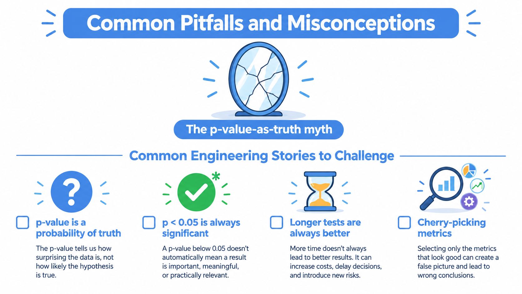
The most damaging statistical mistake is treating a p-value as a truth meter. A p-value is evidence evaluated under a null model. It isn’t the probability that your hypothesis is true, the probability that the release will succeed, or a measure of how important the observed change is.

A result can be statistically persuasive and operationally irrelevant. For example, a checkout change could produce a 0.1% lift that reaches statistical significance at scale but contributes too little practical value to justify its complexity or risk. That example illustrates the difference between statistical significance and practical significance, and the 0.1% figure is used here as a hypothetical illustration, not a reported result.

The review of p-value reliability and replication describes why p-values can vary across repeated samples, particularly when power is limited. Whether a result holds up depends on power, sample size, and design, so a single significant result isn’t a reproducibility guarantee.

Stories that make noisy results look convincing

Peeking creates a tempting feedback loop. A team checks the dashboard repeatedly, stops when the result crosses its threshold, and reports the stopping point as though it had been fixed in advance. The repeated looks change the probability of a misleading threshold crossing.

P-hacking can involve trying alternative filters, outcomes, time windows, or statistical methods until one produces a preferred result. Multiple comparisons create a related problem: testing many metrics or segments makes an apparently unusual result less surprising, even if each individual test looks conventional.

Underpowered tests produce both false alarms and missed opportunities. A non-significant outcome may reflect insufficient information rather than evidence that the treatment does nothing. A significant outcome from a volatile, low-power setup may also be unstable when repeated.

Slicing the funnel introduces another trap. Simpson’s paradox occurs when an aggregate pattern differs from the patterns inside relevant groups because group composition changes. A treatment may look better overall while performing worse for an important device, geography, or customer segment. Segment analysis should follow a reasoned plan, and teams should inspect whether the treatment and control populations remain comparable.

Use habits that make the analysis harder to distort:

• Pre-register the question: Write outcomes, exclusions, thresholds, and the analysis method before reviewing results.
• Fix the horizon: Decide when the test ends and don’t stop solely because the graph looks favorable.
• Protect guardrails: Monitor errors, latency, and operational health alongside the primary metric.
• Review the effect: Ask whether the estimated magnitude matters before celebrating significance.
• Audit segments: Check assignment quality and segment definitions before trusting subgroup conclusions.

Connecting Tests With Monitoring and Next Steps

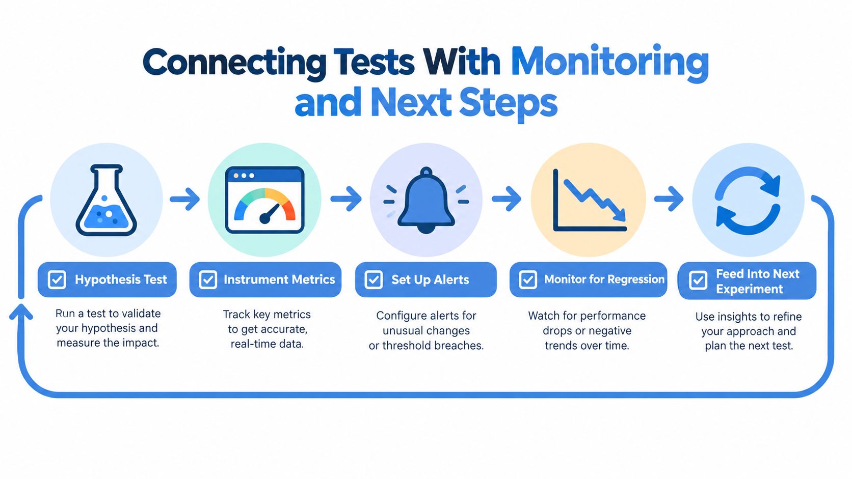
A hypothesis test shouldn’t be the final report card. It should become the first link in an observability loop that continues after launch.

Start with shared metric definitions. If the experiment measures checkout completion, define the event, eligibility rules, deduplication logic, and time window in one place. Feed those definitions into the experiment analysis and the long-term dashboards built with Prometheus, OpenTelemetry, or your analytics platform. Otherwise, the team may ship based on one calculation and monitor a subtly different metric afterward.

Turn the result into an operating loop

Instrument the primary outcome and the guardrails before rollout. Set alerts for operational regressions that require immediate attention, such as rising errors or unacceptable latency. A p-value can’t warn you that a dependency began failing after the experiment ended, but a well-designed alert can.

The GoReplay monitoring documentation can help teams think through replay and service-observation workflows alongside their existing telemetry. Monitoring doesn’t replace inference. It catches changes that occur outside the original test window and supplies evidence for the next investigation.

Use a short post-launch checklist:

• Re-evaluate after two weeks: Treat this as a planned follow-up checkpoint, not a claim that every experiment needs the same schedule.
• Watch for novelty effects: Early behavior may differ while users, caches, or operators adjust.
• Archive raw data: Preserve enough context for later analysis and replication.
• Schedule a retrospective: Convert the statistical result into a product and engineering decision.
• Measure every shipped hypothesis: Assign an owner and a follow-up metric before flipping the feature flag.

The mature habit is simple: every shipped hypothesis gets a follow-up measurement. The original test tells you what the evidence supported under its design. Monitoring tells you whether that conclusion remains useful as traffic, dependencies, and user behavior change.

---

Use GoReplay to capture and replay realistic HTTP traffic against candidate builds, compare behavior before real users are exposed, and connect replay findings to a defensible hypothesis-testing workflow. Visit GoReplay to explore how record-and-replay testing can strengthen your QA, release, and observability process.